By Lorenzo Spisni and Massimo Tassinari Technical advisors for cathodic protection at InRete Distribuzione Energia From the presentation at SMART GRID DAYS 2025, October 8 – 9, 2025.
In the past, we all started from the EON potential data. Then, about ten years ago, we had access to a potential probe that could provide us with additional information. Over time, we discovered that the potential probe could detect the Esonda potential value, coupon current values (Icoupon), and, as we approached the goal of reducing ohmic drops on the potential value, the probe allowed us to obtain EOFF to reach the so-called “free of ohmic drop potential”.
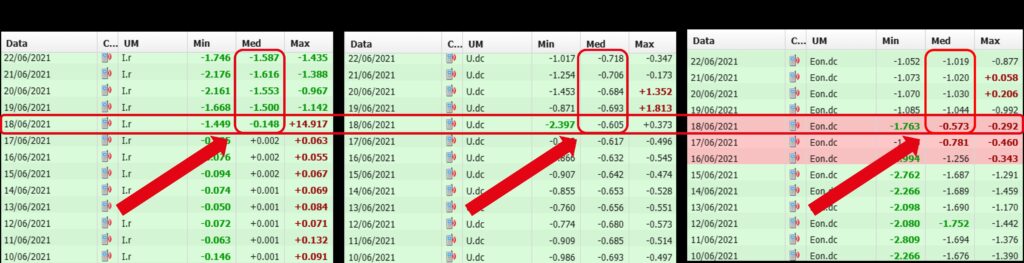
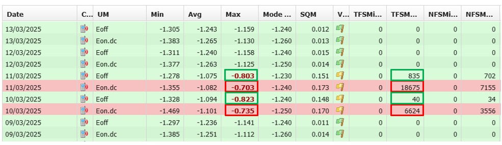
The experience we have carried out on an electrical system is one that gathers a lot of information: we will obtain EOFF measurements on the pipeline and the values of EOFF on coupon. In summary, I would say measurements “with two faces”, as comparing the EOFF measurements obtained with the two techniques proposed by the standards, the data will be conflicting: some data will be compliant and others that probably no one will ‘like’.
Contradictory or ambiguous EOFF values point the way towards more in-depth investigations: these non-compliant data are not due to the reliability of the potential probe product, but we must find the causes in the pipeline – probe – coupon – ground circuit, not forgetting the presence of oxygen.
We will demonstrate that, despite the collected values being conflicting, there are many other basic conditions that completely exclude the possible corrosion of these pipelines.
The regulations and EOFF
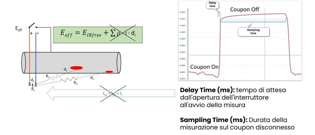
We have definitions both in the standard UNI EN ISO 15589-1 and in the standard UNI 11094. In the latter, two methods for acquiring the EOFF potential are mentioned: directly on the structure with interruption of the cathodic current with a typical delay acquisition of 300 milliseconds or on a plate or probe after opening the electrical connection plate-structure within a maximum time of 100 ms. These techniques are valid for the detailed assessment of the effectiveness of the protection condition.
The technique and utility for testing the electrical system and periodic checks are defined in the standard UNI EN ISO 15589-1 (Appendix A.2.3 – A.2.5 and Art. 7.3 – 12.4.2 and Art. 13.3). Therefore, this information on EOFF is valid both in technical scope (how to do it) and in testing (commissioning or testing the protection condition of a system) and regarding the scheduled maintenance of a system (UNI 11094 Appendix A1, A2, A3).
Thus, the experience we bring transfers the cited regulations within a field context, to obtainEOFFinformation that comes from buried structures.
Below are the techniques adopted for the acquisition of EOFF potential:
directly on the structure (delay of about 300 ms) EOFF-pipe
use of potential probe (within a maximum time of 100 ms) EOFF-coupon
acquisition time of EOFF potential within 2 ms (overprotection),
acquisition time of EOFF potential within 21 ms,
acquisition time of EOFF potential within 100 ms (protection criteria).
We have identified a suitable electrical system, not subject to interference or with a sufficient non-interference period for data monitoring, where the characteristic measurement points were equipped with potential probes.
The system was identified in a small urban area.
The peculiarity of this system is the presence of a different ground resistivity: in fact, there are areas where, following the reclamation of marshy and lagoon areas, the resistivity is around 7-8 Ω·m, while others, formed on fluvial deposits, present a resistivity in the order of 100 Ω·m.
To explore in detail, it is possible to download the complete case study.
Massimo Tassinari is the technical contact for cathodic protection at INRETE Distribuzione, where he is involved in commissioning and supervising the testing of cathodic protection systems, updating monitoring systems and coordinating ARERA data reporting.
By Ivano Magnifico, Product Manager AUTOMA From the presentation “Back to the future: when the past is already the future” SMART GRID DAYS 2025, 8 – 9 October 2025.
Are we using the data we receive from the monitoring systems of cathodic protection as we should? To understand this, let’s summarise the history, the current situation and the future of pipeline monitoring, particularly focusing on what we take for granted and what seems normal because we see it every day.
In this article and the previous one, we talk about monitoring methods and how to optimise data transmission, showing you some concrete examples.
With this content, we are mainly addressing foreign readers, who have different management practices than those we have in Italy. However, in any case, the recap can also be useful for us Italians to see if we are working to the best of our abilities.
Remote monitoring for cathodic protection
For a definition of remote monitoring, please click here.
Let’s now see how the information collected can help us carry out our daily business. In order to have effective and efficient cathodic protection, the first thing to do is to check that the devices we use (e.g. power supplies, decoupling devices, mitigation devices, etc.) are working properly. ISO 15589-1 gives us an indication of the devices that must be checked for cathodic protection:
Cathodic protection rectifiers
Unidirectional drainage station
Connections to third-party structures (resistive or direct)
AC/DC decoupling devices
Galvanic anodes
Measurement points
Rectifier: monitoring parameters
Below are theparameters to be monitored in the rectifier to make sure it is working properly.
DC output current
DC output voltage
AC output voltage: alarm if average value > defined threshold
Presence/absence of main power supply (real-time alarm)
DC potential structure and AC voltage
OFF potential on structure
Instant-off on coupons to measure IR-free potential
DC and AC current density on coupon
When we talk about gas distribution networks within cities, one of the most critical aspects is the life time of the ICCP anode: as long as the ICCP anode is operational, we are able to supply power, but when it wears out, it becomes a problem because it can take up to one or two years to obtain the permits to carry out the work. Therefore, it would be convenient if, in addition to the other information that comes to us, we could also know if and when the ICCP anode is reaching the end of its service life.
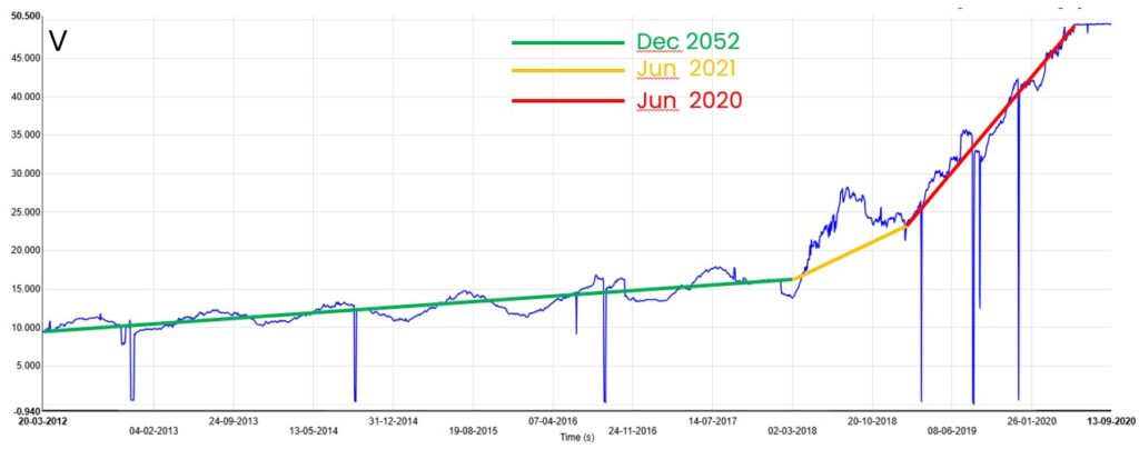
Rectifier: assessing the status of the ICCP anode
In the graph below, we are not measuring impedance (the ratio between voltage and current) to evaluate the total resistance of the circuit, but we are only measuring the output voltage on a rectifier that has always operated at constant current; therefore, the voltage trend follows the trend of the total impedance seen by the rectifier.
The reference period is 2012-2020. Looking at the graph, we clearly recognise the seasonal trend, i.e. the change in soil resistance between the summer and winter periods. However, it is also possible to detect a certain linearity, which is given by the trend of the volume loss of the ICCP anode over time. As we approach the end of service life, we lose this linear trend that tends to become exponential and this can help us predict even a couple of years in advance the moment when a new ICCP anode will be needed.
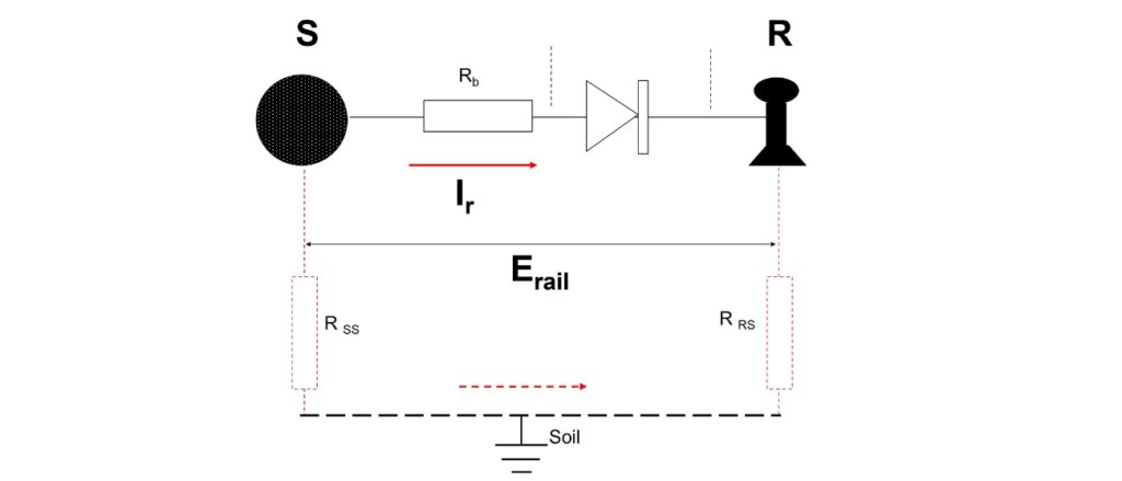
Unidirectional drainage
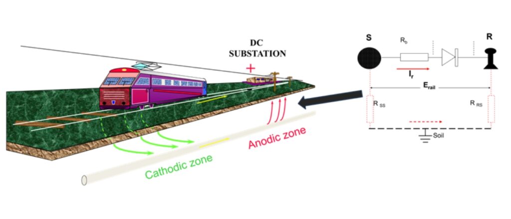
In the vicinity of a railway line, at the point where the interference creates an anode zone of current on our pipe that returns to the original circuit, we will need a drainage, if there are no other ways to solve the problem.
The purpose of drainage is to allow the current, which we absorb in the cathodic area from the railway line, to return via an electrical path to the rail and the substation to which it belongs. Clearly, we only want this current to flow back to the substation and not vice versa.
Another interesting parameter is the potential difference between the structure and the rail: when the structure is more positive than the rail, we expect current to drain, returning to the original circuit; whereas, when the polarisation is reversed, we do not expect current through the diode, because it is reverse polarised.
The monitoring parameters are:
DC drain current
Normal condition: Ir ≥ 0
Alarm if Ir < 0 (damaged diode)
Pipe-to-rail potential (Erail)
Normal condition: -V < Erail < 0.7 V + Ir (Rb+Rpr) (Rpr = parasitic resistance of the diode)
DC potential structure and AC voltage
OFF potential on structure
Instant-off on coupons to measure IR-free potential
DC and AC current density on coupon
Real cases
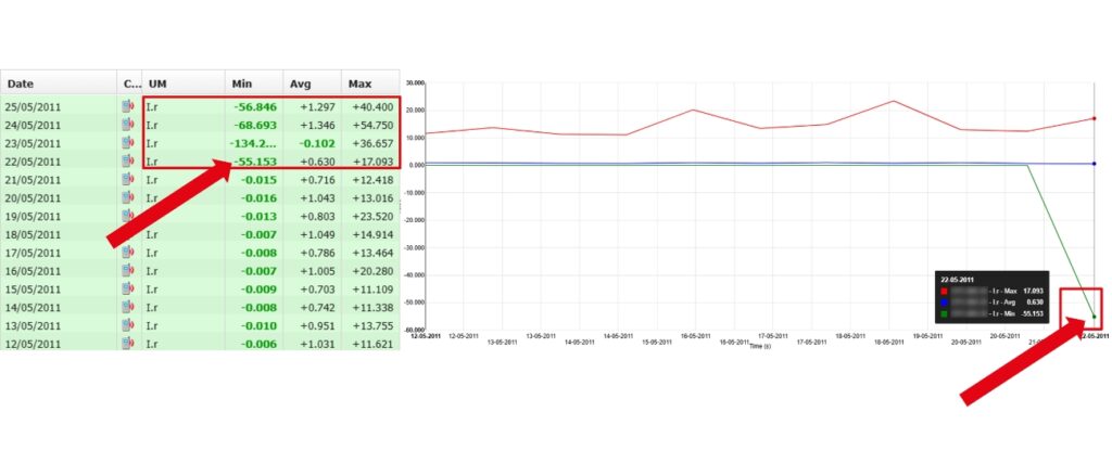
Unidirectional drainage: diode failure detection
Let’s look at some practical examples. Below you see the diode current trend over a series of days; the current flows in one direction only until 22 May. As shown, after the fault, our pipeline is receiving 55A, 134A, 68A from the rail through an electrical connection: this current, however, must return to its original circuit. Generally, corrosion is not a rapid phenomenon, but in this case it can become so. Therefore, it is essential to receive an alarm so that prompt action can be taken.
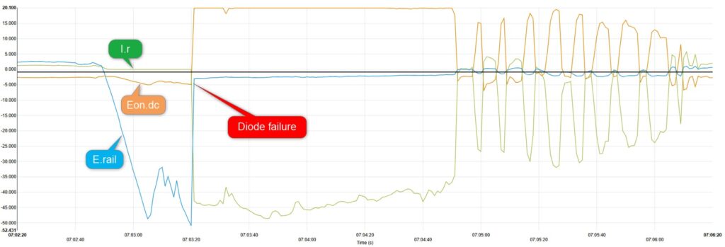
With reference to the Remote Datalogger Unit, it is interesting to point out that we can occasionally ask the device to download the measurement second by second in order to analyse in detail what happened; and that is what we did in this example. We downloaded the intensive measurement per second on the day the diode broke. Below we can see the drained current, the On potential and the tube-rail potential.
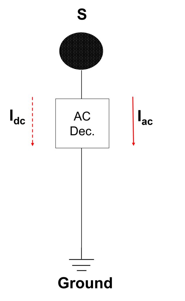
AC mitigation device: monitoring parameters
The AC decoupler is a large capacitor between the pipe and the grounding system, which allows the AC current to be discharged to the grounding system while remaining an open circuit for the DC current.
What do we monitor?
AC current discharged;
DC current:
Normal condition: average IDC= 0
Alarm if average IDC ≠ 0 (damaged decoupler, presence of resistive path)
Grounding potential (Egnd):
Alarm if Egnd drops to more negative values;
DC potential on structure and AC voltage;
OFF potential on structure;
Instant-off on coupon to measure IR-free potential;
DC and AC current density on coupon.
AC mitigation device: fault detection
The daily report shows the direct current recorded over several days, until the day when the average value becomes different from zero.
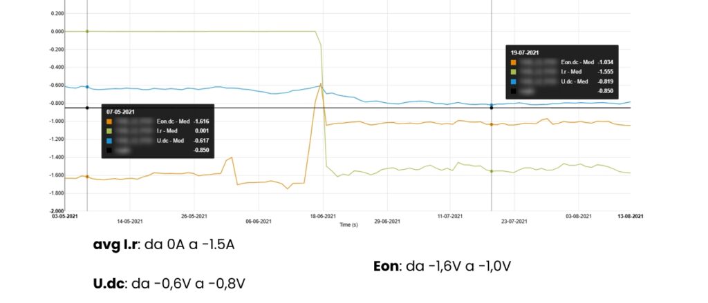
Taking the potential of the grounding system into consideration, we see that the variation is slight; this is because the ground network is very extensive and a lot of current is needed to generate a significant variation in potential. Instead, looking at the graph on the right, one can see that the potential varies greatly, going from -1.7 V to -1 V. In this case, we are far enough away from the rectifier that it does not realise that something is drawing current.Therefore, the rectifier continues to operate, losing 600-700 mV on the ON potential.
Therefore, we can identify the day and detect the presence of the fault, also analysing the temporal trend. This is important because if I have to do a historical analysis of the data – not only on this measurement point but on the other points of the system – having a signal that allows me to understand when the alternating current discharge device was not working properly also allows me to correlate the other values.
Effective cathodic protection
To ensure that cathodic protection is effective, ISO 15589-1 defines two steps:
General assessment
ON potential measurements performed on all measurement points or at least on selected ones.
Detailed and comprehensive evaluation
OFF potential measurements preferably carried out at all measurement points.
When an OFF potential measurement on the pipe is not possible, OFF potential measurements are required using probes or coupons at significant time intervals.
The NACE SP0169 standard, which is equivalent to 15589-1, establishes the following criteria:
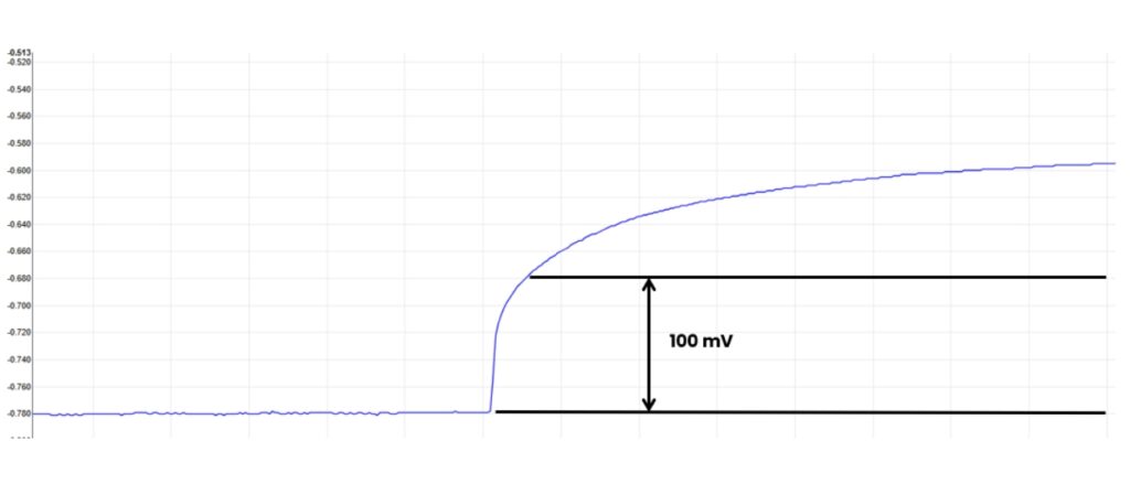
A minimum of 100 mV cathodic polarisation.
Structure-electrolyte potential equal to or more negative than -850 mV relative to a copper/copper sulphate saturated electrode (CSE).
This potential can be a direct measurement of the polarised potential or an ON potential.
Use of cathodic protection coupons to establish current density levels, corrosion potential, polarisation levels.
Evaluation of ON potential
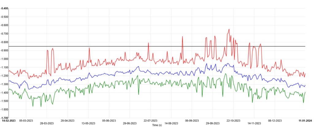
The graph below shows that we are protected during the year. There is, however, a period when the daily maximum is out of protection. This does not mean that we are in a serious risk of corrosion, because we must also evaluate the other information provided by the daily report (e.g. time out of protection).
Instant-off potential on coupon
Measurement Technique
We perform the instant-off measurement with the coupon and manage to eliminate the IR drop. This is a measurement that we can do simply by taking the instant-off values: it is done over a few milliseconds and we can repeat it once per second. Therefore, we have a 1-1 ratio between instant-off potential on coupons and ON potential.
Daily report
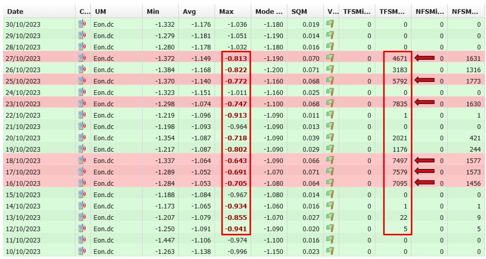
In the report below we see the measurement points, the out-of-protection maximums, and the out-of-protection times. In this case, the time out of protection of the ON potential is between two and five hours. So I might be induced to go into the field to find out what is going on.
As I mentioned earlier, here we are assessing whether we are cathodic or not;we are unable to know what the IR-free potential is to compare with the criterion we apply. Coupons help us: if we take into consideration those same days and the instant-off measure on the coupon where we eliminated the IR, we see that the real time out of protection is negligible.
In a set of measurements where I may have several points where the ON potential is unprotected, the coupon measurement allows me to filter out all those points where there is actually only an ohmic drop in the ground and analyse where there is a real need.
100 mV shift
Having the coupon and being able to control it remotely, we can also evaluate the 100 mV shift criterion: I can download the measurement second by second and make the evaluation.
DC interference
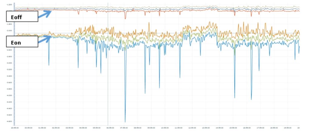
The graph below is interesting because we have the 24-hour ON potential and the instant-off potential on coupon. Having both measures allows us to assess the effect of interference. Looking at the night phase, the two lines are practically parallel. During the passage of trains, however, the ON potential chases all the currents circulating in the ground – these currents do not necessarily enter our structure. Therefore, the possibility of evaluating the two curves in parallel allows us to understand when the interference generates currents only towards the ground and when it also generates them towards the structure, resulting in cathodic and anodic conditions.
ON potential vs. instant-off on coupon
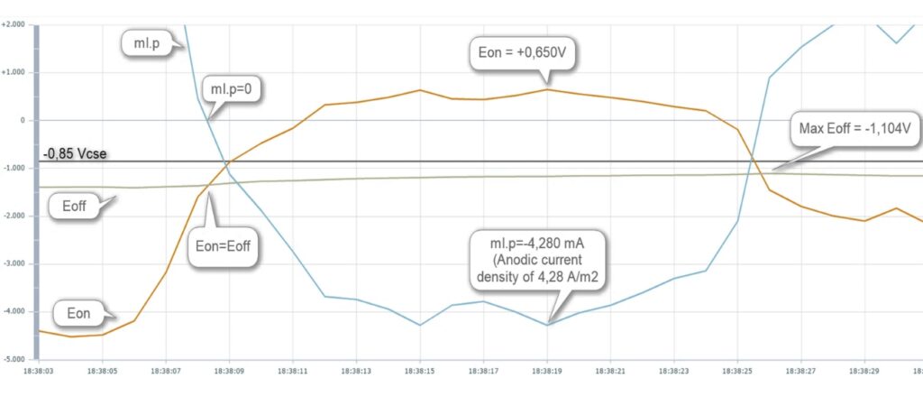
In the image below we report an example that is very interesting. In an interference condition, I download the measurement second by second. We have 30 seconds of measurement in which there are the ON potential and the current in the coupon. The current in the coupon when cathodic is positive and when anodic is negative. Thus, here we have the effect of an anodic interference that lasts approximately 15 seconds, with a maximum peak of 4 A/m2. Therefore, we have: anodic interference, 4 A/m2 current density, and positive ON potential (+ 0,65V CSE).
The first action one is tempted to take to eliminate a positive potential is to increase the current. However, in this case, by analysing the average daily values, we are heavily overprotected (-1.3 V CSE), so going to increase the current would make the situation even worse.
This is where the point we were making earlier comes into play: the importance of being able to assess the time out of protection. This is because if over the course of 24 hours the structure is protected, 30 seconds of anodic interference is not enough to generate a risk of corrosion. If we were instead to evaluate the instant-off potential during this interference, the most positive maximum value we would reach is -1.1 V. Therefore, it would be harmful to increase the current. If the rest of the cathodic protection system allowed it, we could even consider reducing the current slightly and attempting to exit the overprotection condition.
Therefore, depending on the quality and type of information I receive, I may even be led to make completely opposite choices, but at the risk of making the wrong ones. The more information I can obtain, the more convinced I will be of my actions because they are supported by data –reducing the probability of error.
AC interference
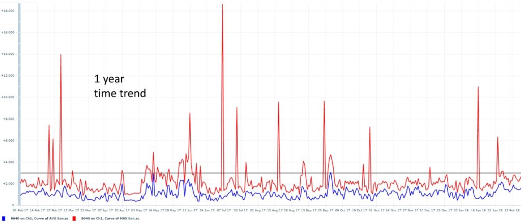
Alternating interference is rather insidious, as it is highly dependent on ground conditions. Soil conditions can vary throughout the year: a compliant measurement at a certain time of the year does not guarantee – unless I have continuous monitoring – that it will be equally compliant at another time of year.
If, in this case, the technician were to take a measurement, he would find 1.5 V of AC voltage. However, the graph below shows that there are times of the year when even 15 V is exceeded. With continuous monitoring I can get this information.
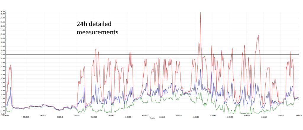
The graph below shows what can happen in industrial areas. Shown below is a 24-hour intensive measurement in an industrial area where there is probably a company with machinery with poor ground insulation. Therefore, we can count the machine cycles they are performing within 24 hours, and this may help us identify the source and request a solution to the problem.
The AC density is very sensitive to changes in ground resistivity. So – given the same external conditions – I can have periods of the year when the density is above 30 A/m2, others when perhaps, with a higher resistivity (summer period), the density drops dramatically and then goes back up again.
The monitoring configuration in the presence of alternating interference becomes quite critical. What we can measure is:
DC ON potential on structure and AC voltage;
Instant off potential on DC coupon (10 cm2 or other size, for evaluation of the protection criterion)
DC coupon current density
DC and AC current density on AC coupon (1 cm2)
With this setup I can check the following criteria:
-1.2V CSE < Instant off potential on coupon < -0.850V (according to ISO 15589-1 and SP0169)
Average daily AC voltage < 15 Vac (according to ISO 18086 and SP0177)
Daily average of Jac < 30 A/m2 (or Jac < 100 A/m2 if daily average Jdc < 1 A/m2) (according to ISO 18086 and SP21424)
In this article and in the previous one we have seen something that for Italy it has been history for 25 years. The ability to integrate remote monitoring features with high-frequency measurement monitoring, typical of data loggers, allows – in the presence of local intelligence capable of processing such data – intelligent reporting, evaluation, and simple detection of conditions that are normally difficult to detect.
The technician does not disappear in this activity, but he stops being a driver: he can spend more time in the office, analysing concrete data and dealing with abnormal conditions – having consistent data. At a time when human resources tend to be increasingly scarce in various cathodic protection groups, this type of assistance becomes essential for optimising all our activities.
Like Marty McFly in 1955,the rest of the world is finally reaching a future that for us has already been present for a quarter of a century. Italian technology has been the DeLorean, bringing innovation where it seemed impossible.
AUTOMA designs and produces innovative, Made in Italy hardware and software solutions for remote monitoring and control in the Oil, Gas and Water sectors.
We were born in 1987 in Italy, and today over 50,000 Automa devices are installed in more than 40 countries around the world.
Do you want to know the benefits for the security of your networks that you could have with the AUTOMA monitoring system for cathodic protection?
Contact our team without obligation and we will tell you what we can do to optimise your infrastructure control.
Electronics engineer, he is certified as a Senior Technician in cathodic protection and specialises in market analysis and industry standards. With more than 15 years of experience in remote cathodic protection monitoring and a patent on an intelligent reference electrode, Ivano is a member of the Board of Directors of Ceocor (European Committee for the Study of Corrosion and Protection of Piping Systems) and Delegate of AMPP Italy Chapter, as well as an active member of the ISO and AMPP standard working groups for cathodic protection.
By Ivano Magnifico, Product Manager AUTOMA From the presentation “Back to the future: when the past is already the future” SMART GRID DAYS 2025, 8 – 9 October 2025.
Are we using the data we receive from the monitoring systems of cathodic protection as we should? To understand this, let’s summarise the history, the current situation and the future of pipeline monitoring, particularly focusing on what we take for granted and what seems normal because we see it every day.
In this article and the next, we will talk about the monitoring methods and how it is possible to optimise data transmission.
With this content, we are mainly addressing foreign readers, who have different management practices than those we have in Italy. However, in any case, the recap can also be useful for us Italians to see if we are working to the best of our abilities.
Definition of Remote Monitoring
UNI EN ISO 15589-1:2017 proposes this definition of remote monitoring: “At a minimum, remote monitoring must provide the same level of information obtained by cathodic protection operators in the field”.
What does this mean? The “minimum” is a precise measurement taken at the same frequency with which a technician can go out into the field to carry out checks. Relying solely on this standard means taking things a bit too literally: you can imagine what it means to take a precise measurement every six months, considering everything that can happen in the meantime.
There is no definition of remote monitoring in the NACE standards. However, there is a working group that has the task of drafting the MR21551 standard on remote monitoring. When this standard is drafted, you will find that there is some reference to what we do in Italy.
RMU vs Datalogger
When we limit ourselves to what the standard requires, we are faced with a contrast between what a remote monitoring unit (RMU) does, which takes measurements from time to time, and what a data logger does, which analyses the effects of interferences with high-frequency measurements. Normally, one faces a dilemma: which one to choose?
If we choose a remote monitoring unit, we limit ourselves toperiodic measurements withlow transmission requirements, but we forego high-frequency sampling. If we choose adata logger, we will have high sampling frequencies and an assessment of transienteffects, but data retrieval will be difficult and usually done manually, as the device does not have remote access.
ON potential trend on structure
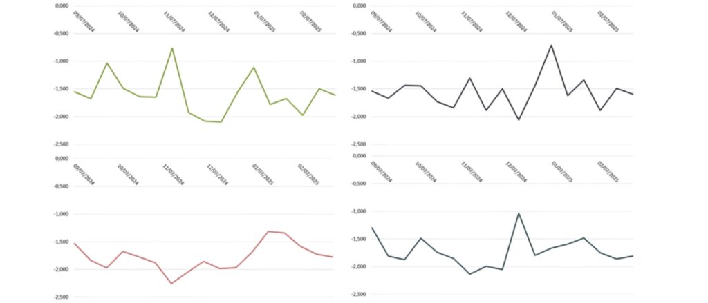
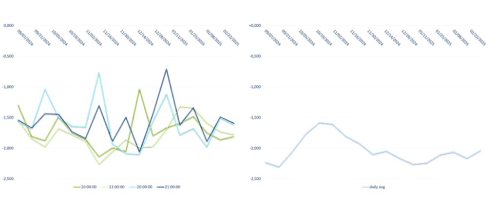
This graph shows four potential trends at four measurement points over six months (one measurement per week).
These measurements appear to belong to different cathodic protection systems, but in reality these curves derive from the exact same measurement point but relate to different times: we have the curve for 10:00, 13:00, 20:00 and 21:00 (in the figure below on the left). Therefore, this is what I get when I make a precise measurement with a certain periodicity. I lose track of everything that happens in the meantime: I cannot get clear information on the actual trend, which is what can be seen in the graph on the right.
Remote Data Logger Unit and Edge Computing
To overcome this problem, we need a tool that combines the features of a Remote Monitoring Unit (RMU) and a data logger: a Remote Data Logger Unit. This is a device that not only allows us to combine remote communication with high-frequency monitoring, but is also intelligent, highlighting only the key aspects of the information (indeed, there are constraints in terms of the amount of data that can be sent). The goal is to optimise transmission.
This goal can be achieved through edge computing: a computing model that processes information locally and sends only essential data to the Cloud (daily report). It is therefore a device that, like a data logger, can take one measurement per second at the site where it is placed. With this measurement frequency, at the end of the day, 86,400 measurements will be obtained: being a very high quantity, it is unthinkable to send them all, especially since the device runs on battery.
Therefore, the device processes this information and provides a summary, indicating:
Daily minimum, average, maximum: where the average value is a consistent value derived from one measurement per second over the course of the day, making it possible to understand the actual trend (not as in the previous graph on the left).
Statistical information:trend, i.e. the most frequent value measured within the 86,400 samples; standard deviation; and variability, to get an idea of how much the measurement varies throughout the day.
Total time (seconds) below the minimum threshold and above the maximum threshold during the day: to have a range in which to consider the signal valid or invalid; in the latter case, there will be a series of alarms or conditions to pay attention to.
Total number of exceedances of the minimum threshold during the day.
Total number of exceedances of the maximum threshold during the day.
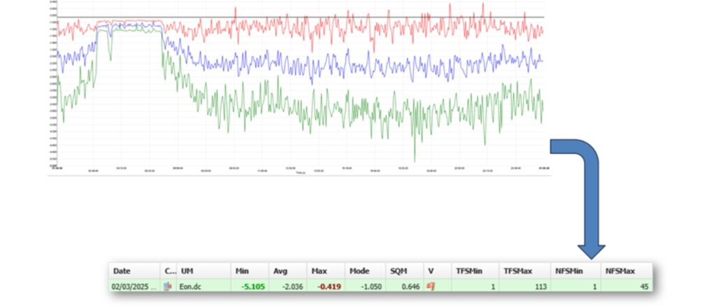
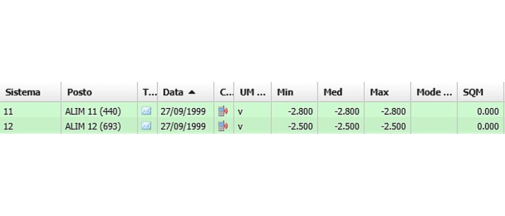
All this information, which is summarised in sets of numbers (see figure below), is contained in few kilobytes of data per day but tells the story of everything that happened over the 24 hours, and it will do so as long as the device is installed.
Read the daily report
Edge Computing
In the figure, we see in detail some values.
Min, avg, max
How can we transform the recording of 24 hours of data into a daily report?
First of all, we have the following information:
Minimum value: the most negative value measured over 24 hours;
Average value: given by the arithmetic mean of the samples taken over 24 hours;
Maximum value: the most positive value measured over 24 hours.
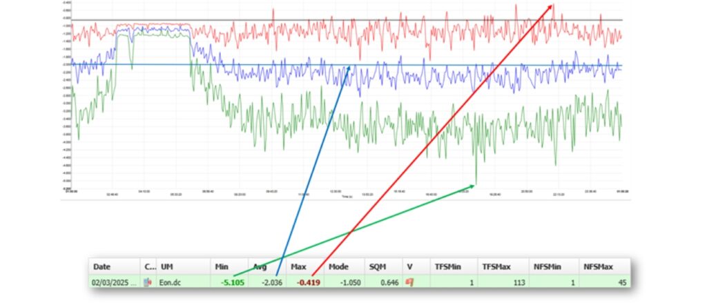
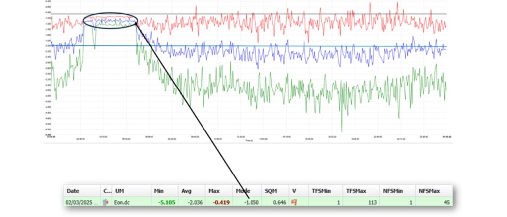
Moda
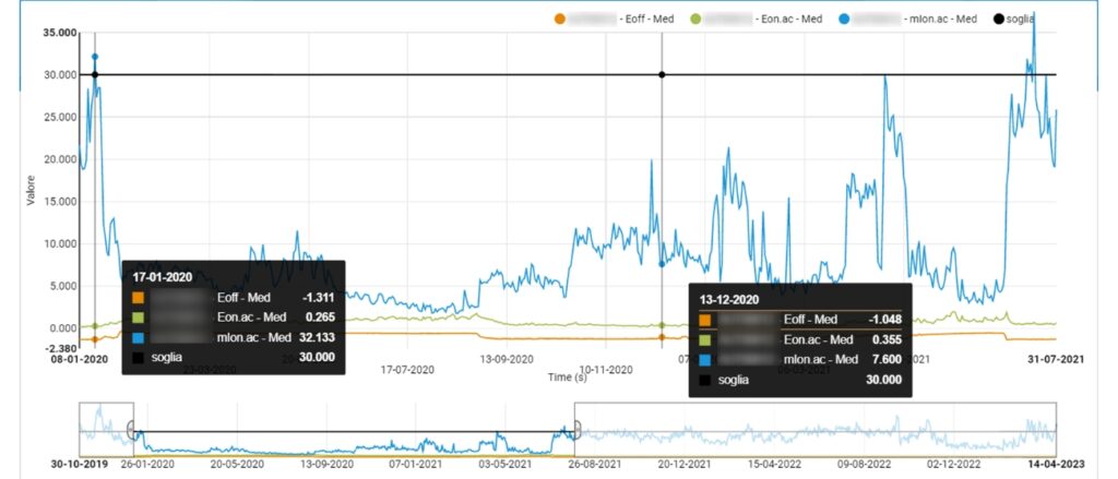
Arithmetically, trend is the most frequent value within a set of samples (86,400 seconds). Usually, mean and trend have similar values, but when we are faced with a non-stationary interference, such as at a railway crossing (see fig. below), the trend takes on a very particular meaning: during the night hours, we find a slightly more stable measurement range and, almost always, the trend value coincides exactly with the value during the night when the system is not interfered with. Indeed, it is more likely that a value will appear consistently multiple times within that range.
So, even in a condition where there is considerable variability, it is possible, from these few numbers, also extract information about what the potential is – in the absence of interference – relative to that measurement point.
Standard deviation and variability
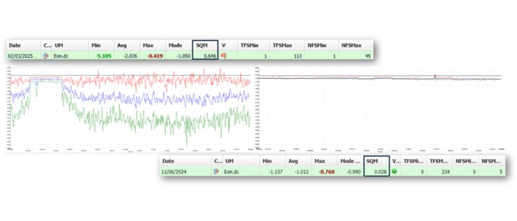
Looking at the type of graph in the figure below on the left, we would expect the standard deviation (or Mean Square Deviation, MSD) to be quite high. I could have measurements with similar minimum and maximum values, but perhaps due to a single interference that lasted only a few seconds.
This can be seen from the standard deviation value; indeed, this value indicates how stable my sample population was over the course of 24 hours. Therefore, even if I have rather wide minimum and maximum values as a range, if I realise that I have a low standard deviation (below 0.05), I know that in reality, throughout most of the day, my value has been close to the average value.
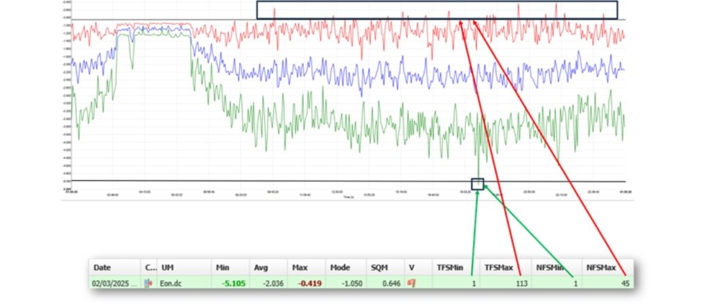
Time and number of alarms
The daily report also allows us to know how long we have been outside the limit conditions we have set.
The minimum out-of-threshold time and the minimum out-of-threshold number provide an overview of how many times you went below that value: in the case shown in the image below, the minimum out-of-threshold was reached once for 1 second. On the other hand, the maximum out-of-threshold time and the maximum out-of-threshold number show how many times one wentabove that value: in the case below, a total maximum out-of-threshold time of less than 2 minutes was reached in forty-five intervals. This, by the way, gives us an idea of the average time out of protection; in this case, we are around 2.5 seconds.
Why is it crucial? Because by takingcontinuous measurements, I canfind out everything that is happening, and I only need to look at this value to check whether the structure is at risk of corrosion. It is clear that in a condition of continuous cathodic protection, small intervals outside the protection levels do not entail an immediate risk of corrosion: it is up to the technician to decide and set the interval above which it is necessary to be alerted. In any case, in Italy, the regulation has established a maximum value of 3,600 non-continuous seconds.
According to ChatGPT, the term “Edge Computing” started to be known from 2014, but became commonly used around 2017. It is important to note this for a simple reason: everything we have seen so far is what has been done in Italy since 2001 as required by the UNI 10950 standard published that year.
In the chart below is the first daily report found in our database, which dates back to 1999, proving that we have been doing Edge Computing “without knowing it” for more than 25 years.
AUTOMA designs and produces innovative, Made in Italy hardware and software solutions for remote monitoring and control in the Oil, Gas and Water sectors.
We were born in 1987 in Italy, and today over 50,000 Automa devices are installed in more than 40 countries around the world.
Do you want to know the benefits for the security of your networks that you could have with the AUTOMA monitoring system for cathodic protection?
Contact our team without obligation and we will tell you what we can do to optimise your infrastructure control.
Electronics engineer, he is certified as a Senior Technician in cathodic protection and specialises in market analysis and industry standards. With more than 15 years of experience in remote cathodic protection monitoring and a patent on an intelligent reference electrode, Ivano is a member of the Board of Directors of Ceocor (European Committee for the Study of Corrosion and Protection of Piping Systems) and Delegate of AMPP Italy Chapter, as well as an active member of the ISO and AMPP standard working groups for cathodic protection.
By Lorenzo Maggioni. From the speech at SMART GRID DAYS 2025 (8-9 October 2025), organised by Automa.
The European context: energy security and the acceleration of biomethane
In recent years, biomethane has assumed an increasingly central role in European energy strategies. Rising gas prices, also triggered by geopolitical tensions between Russia and Ukraine, have highlighted the need to diversify sources and reduce dependence on imports.
Within this framework, the REPowerEU plan has set an ambitious goal: to increase biomethane production to around 35 billion m³/year by 2030. Italy, through its own NECP, aims to achieve 5.7 billion m³/year by 2030, focusing primarily on the conversion of existing biogas plants and the development of new plants.
Figure 1 – Combined biogas and biomethane production and number of plants in Europe (Source: EBA Statistical Report 2024).
Biogas and biomethane in Europe: plant trends and prospects
The European system starts from a plant base historically oriented towards electricity production from biogas. For many years, anaerobic digestion has been driven by incentive schemes linked to electricity generation, with Germany and Italy as the reference markets in terms of the number of plants and the maturity of the supply chain.
Today the trend is different: while the number of new biogas plants for electricity generation tends to stabilise, the number of plants (new or converted) intended for the production of biomethane through upgrading is constantly growing. The expected trajectory in the coming years is therefore a progressive shift in production from biogas ‘power’ to biogas ‘gas’ (biomethane), with increasing integration into networks and end markets.
Biomass and feedstock: evolution of input matrices
The composition of biomass used for anaerobic digestion is a key indicator of the evolution of the sector. In Europe, the predominant share comes from agricultural resources, a category that includes both dedicated crops and, increasingly, livestock effluents and agricultural and agro-industrial by-products.
Historically, especially in the early years of its development, anaerobic digestion in agriculture has relied significantly on energy crops (e.g. corn silage), sometimes in monoculture or double cropping regimes. With the progressive refinement of sustainability criteria and the evolution of policies, the sector has reduced the incidence of dedicated crops, increasing the use of wastewater and by-products, with benefits both environmental and territorial acceptability.
In electric biogas, in addition to agricultural sources, landfill gas plays a significant role. In biomethane, however, the role of landfills is limited (due to the greater complexity of purification), while OFMSW (Organic Fraction of Municipal Solid Waste) assumes increasing importance. In Italy, there are industrial-scale plants powered by OFMSW, with production in the order of thousands of m³/h.
Figure 2 – Distribution of European biogas and biomethane production by type of plant (Source: EBA Statistical Report 2024).
The Role of Incentives: Why the Market Grows in Spurts
As was the case with biogas electricity in the initial phase, the development of biomethane is also strongly correlated with the presence of support mechanisms. Historical data show that production growth has occurred most rapidly in countries that have established stable and bankable incentive schemes.
Germany was the first to launch a structured biomethane industrial supply chain; Denmark, the United Kingdom, and France subsequently achieved significant growth thanks to dedicated national policies. At this stage, Italy is contributing increasingly, especially as a result of the Ministerial Decree of 15 September 2022, which has activated a large portfolio of projects in the ranking.
Figure 3 – Growth in biomethane production in Europe by country (Source: S&P study, as reported in the presentation).
Goals for 2030: NECP, production gap and new decrees
To outline medium- to long-term trajectories, it is useful to refer to the national NECPs, which set targets for 2030 in terms of biogas and/or biomethane production. In the Italian case, the target is 5.7 billion m³/year.
The Ministerial Decree of 2 March 2018 supported the production of biomethane for transport (advanced biofuel), bringing production to values close to 800 million m³/year. With the Ministerial Decree of 15 September 2022 (‘Ter’ biomethane), the total quota is 257 thousand Sm³/h, approximately 2.1 billion m³/year, allocated through five competitive procedures.
Based on the progress made in obtaining authorisations and implementing the projects, it is realistic to expect full-scale production in the order of 1.6-1.8 billion m³/year for this decree. This results in a gap with respect to the NECP target, which makes the introduction of a further measure (often referred to as ‘Quater biomethane’) plausible to support growth in the second part of the decade.
Figure 4 – Biomethane targets in European NECPs and production potentials by 2030 (Source: presentation table, based on NECP data).
Access to gas networks: European principles and operational challenges
Injecting biomethane into the grid is a key step in scaling up the sector, but it requires clear rules and efficient procedures. The new European framework for decarbonised gas markets (Directive (EU) 2024/1788 and Regulation (EU) 2024/1789) strengthens the principles of non-discriminatory and transparent access to infrastructure.
In practice, network operators are required to manage connection requests according to defined and public technical and economic criteria. Any denials or limitations must typically be motivated by infrastructure safety constraints or economic efficiency considerations, within a perimeter subject to the oversight of the National Regulatory Authority (NRA), which can intervene in the event of disputes.
However, an element of fragmentation remains: gas quality requirements for injection are not yet fully harmonised at European level. Differences between countries in parameters such as oxygen, CO2, sulphur, or odorisation impact upgrading design, costs, and, in some cases, the replicability of standard solutions.
Figure 5 – Network connection process for biomethane projects: phases and principles (Source: EBA, 2024).
Gas quality: variability of national limits
The following tables highlight the differences between national gas quality specifications in different European countries. For the operator, these deviations translate into different design requirements (e.g. on oxygen control and sulphur compounds management), with impacts on CAPEX, OPEX and operational reliability.
Figure 6 – Examples of quality requirements for network injection in some European countries (Source: Marcogaz, 2023).
The Italian case: installed base, transition and regulatory pillars
Italy is Europe’s second-largest biogas market, with approximately 2,000 electric plants and an installed capacity of around 1,350 MW. At the same time, approximately 150 biomethane plants are operational, with a production of close to 800 million m³/year (MD 2018 scope).
A strategic issue is linked to the life cycle of historical incentives: over 1,100 electrical systems built with particularly favourable tariffs (e.g., 0.28 EUR/kWh, with a 15-year duration and entry into production between 2009 and 2012) will reach the end of their incentive period in 2027. Without transition tools, a significant portion of plants risks exiting the market.
In this context, the legislator has chosen to orient the supply chain towards the production of biomethane, introducing two key decrees (MD 2/3/2018 and MD 15/9/2022) and completing them with further provisions and technical standards. In particular, today the sector is based on three pillars: Ministerial Decree 09/15/2022 (incentives), MD 224/2023 (Guarantees of Origin) and Legislative Decree 63/2024 (contractual instruments and integration with industrial demand).
Figure 7 – The three regulatory pillars of biomethane in Italy: incentives, GOs and contractual instruments.
Ministerial Decree 15/09/2022: incentives, competitive procedures and NRRP
The Ministerial Decree of 09/15/2022 provides for two incentive methods: an all-inclusive tariff and a premium tariff, depending on the sale/collection configuration. Access is via competitive procedures (auctions), and the total allocable quota is equal to 257 thousand Sm³/h, equivalent to approximately 2.1 billion m³/year.
A highly attractive element is the NRRP’s capital incentive, up to 40% of the investment cost within the established ceilings. Furthermore, the decree extends the intended use of biomethane to applications other than transportation, opening up the industrial market in a more structured way.
In competitive procedures 3-5, the reference tariff is 124.48 EUR/MWh (value indicated by the decree and the application procedures). The result is a portfolio of 554 ranked projects, which has employed approximately 90% of the available quota.
Figure 8 – Summary of projects in the ranking (MD 09/15/2022): number, capacity, types and territorial distribution.
GO and industrial demand: MD 224/2023 and LD 63/2024, art. 5-bis
Ministerial Decree 224/2023 regulates the issuance of Guarantees of Origin (GO) for biomethane. The GO is an electronic certificate that attests to the renewable origin of production: in the absence of a GO, the gas fed into the network is indistinguishable — in terms of “claims” — from fossil gas.
The LD 63/2024 (known as the ‘Agriculture Decree’), in Article 5-bis, introduces the possibility of bilateral agreements between agricultural biomethane producers and hard-to-abate industries. In this configuration, GO can be transferred to the final consumer, with potential applications within the ETS scope as a tool for decarbonisation and, in fact, industrial competitiveness. In practice, part of the economic benefit can be shared along the supply chain, contributing to the bankability of the projects.
UNI technical standards: gas quality and sustainability criteria
On a technical level, UNI/TS 11537:2024 defines requirements and verification methods for the quality of biomethane intended for injection into the network. UNI/TS 11567:2024, on the other hand, details the criteria and methods for calculating sustainability, with particular attention to the reduction of climate-altering emissions (GHG) along the entire supply chain.
To qualify for incentives, biomethane must demonstrate a reduction in emissions compared to benchmarks: for transport, the benchmark is 94 gCO₂eq/MJ with a minimum reduction of 65%; for other end uses, the benchmark is 80 gCO₂eq/MJ with a minimum reduction of 80%.
Figure 9 – Comparison of national gas quality specifications in Europe (Source: Marcogaz, 2023).
Conclusions: an accelerating supply chain
The European regulatory framework (RED III and Gas Package) and the evolution of national instruments are making the growth context for biogas and biomethane more defined. In Italy, the large base of biogas power plants provides a unique opportunity to accelerate the conversion to biomethane and contribute substantially to the NECP and European targets.
The combination of incentives (MD 15/09/2022), traceability and valorisation tools (GO), and new contractual models with industrial demand opens up concrete development prospects. This is accompanied by economic and employment effects, with an expected increase in green jobs along the entire value chain: plants, agricultural supply chains, services, engineering, and the technology industry.
Figure 10 – Evolution of decrees and targets for 2030 (source: summary slide from presentation).
Lorenzo Maggioni, PhD, is an Italian agronomist and senior advisor with over 20 years of experience in the renewable energy sector, specialising in biogas, biomethane and bioLNG. Formerly head of research and development and biomethane manager at the Italian Biogas Consortium (CIB), he has led EU projects (BIOSURF, REGATRACE, SABANA, ISAAC) and contributed to the Italian policy framework on biomethane. Today, he advises investment funds, energy companies and institutions on plant development, sustainability certification and regulation. He has collaborated with the Italian National Research Council, lectures at the Rome Business School and speaks internationally, promoting sustainable biomethane solutions for energy transition and decarbonisation.
Written by Tommaso Russo, Product Manager Area of the AUTOMA Sales Division From the intervention “A solution for the quantification and reduction of methane emissions” SMART GRID DAYS 2025, 8 – 9 October 2025.
Monitoring and reducing emissions efficiently are an urgent necessity, not only from an environmental perspective but also from a regulatory one.
Regulation (EU) 2024/1787 marked a turning point for the energy sector. For the first time, the reduction of methane emissions becomes a structured obligation, with precise deadlines and requirements that affect the entire gas supply chain: transport, distribution, storage and regasification.
The regulatory framework, however, is developing in a complex context. The deadlines are tight, the requirements are increasing, and not all of the technical tools supporting the Regulation are fully available yet. Operators are thus faced with having to make operational and investment decisions in an evolving scenario, where regulatory uncertainty is compounded by the practical difficulties of effectively measuring, quantifying and reducing emissions.
It is precisely in this context that a key need emerges: to have solutions that allow us to move from theoretical estimates and sporadic campaigns to continuous and reliablecontrol that can also be used for future compliance purposes.
From detection to emissions management: the limitations of traditional approaches
Today, the search for methane leaks is based mainly on LDAR campaigns carried out with OGI cameras and portable FIDdetectors. Fundamental tools, but which have structural limitations.
Firstly, the frequency of inspections is limited: the LDAR (Leak Detection and Repair) programme is carried out every three or even six months, and leaks could occur during these intervals.
Another important limitation is human bias: the operator could make mistakes when detecting leaks or may not detect them all. Last but not least, the accessibility of components can also represent a problem: often stations have rather complex configurations and, therefore, components with high leakage rates may not be detected.
Even the quantification of emissions, often based on generic emission factors and inventories that are not always updated, returns an approximate picture, which tends to underestimateactual leaks. This approach may be less and less adequate in the light of new regulatory requirements, which require more representative and verifiable data.
In terms of reduction, available solutions often impose operational compromises: replacement of components with impacts on service continuity, reduction of operating pressure with the risk of not meeting network demand, or difficult or impossible interventions on inaccessible leaks. In the absence of zero-loss components, it becomes apparent that the problem cannot be addressed with a single approach.
MethanEye: monitor and quantify to make better decisions
MethanEye was created with a specific objective: to provide operators with a reliable tool for the continuous monitoring and quantification of methane emissions, transforming a regulatory obligation into an opportunity for control and optimisation.
The device integrates a CH₄ sensor capable of detecting concentrations in ppm and converting them into emissions expressed in kg/year, as required by regulatory requirements. Thanks to its compact design and installation in ATEX zone 0(methane and hydrogen), MethanEye can be placed directly near the source, intercepting even hard-to-reach leaks.
The flexible power supply — from the network, solar panel or battery — allows installations even in remote locations, ensuring almost continuous monitoring (sampling every 30 seconds) or configurable according to operational requirements and the required duration. The result is a constant flow of data, which reduces uncertainty and supports decisions based on real evidence, not on estimates.
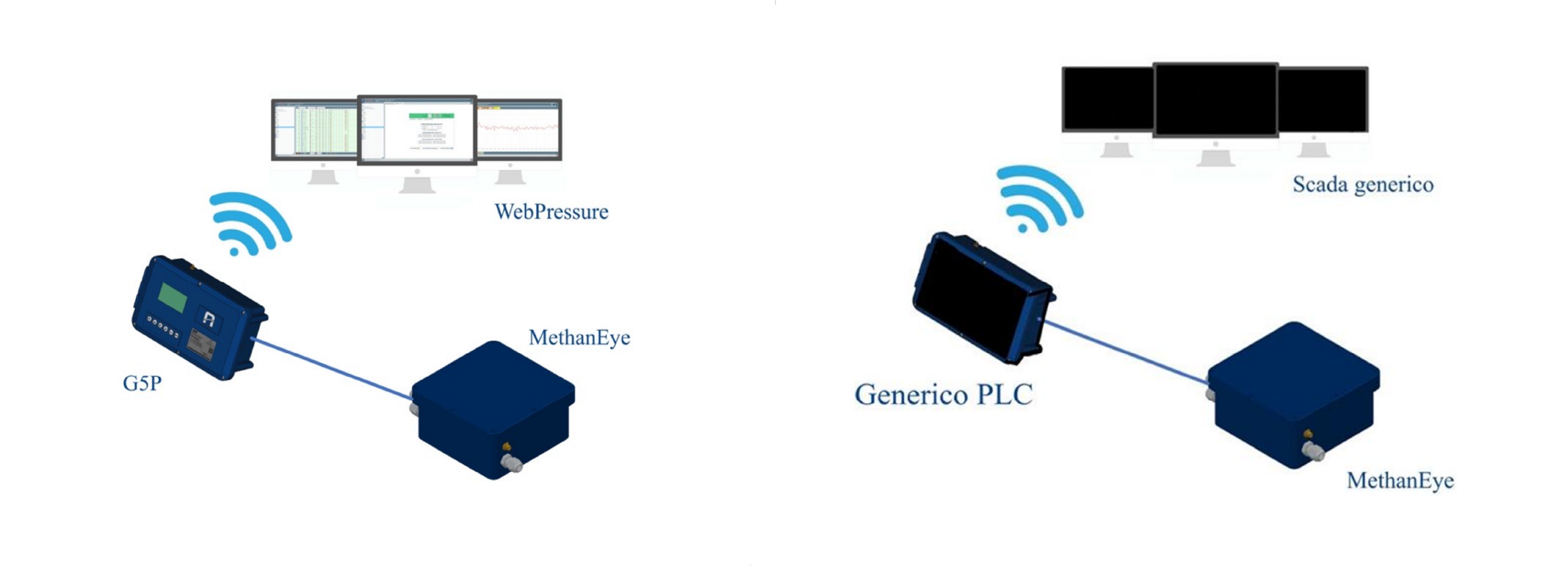
MethanEye can easily integrate with existing PLC, G5P Automa and SCADA systems, or operate in stand-alone mode thanks to the integrated modem. This flexibility makes it suitable both for new installations and for the adaptation of existing systems.
Reducing emissions without compromising the network: GOLEM-ZERO
Measuring and quantifying is essential, but not enough. The reduction of emissions also involves a more intelligent management of operating conditions. GOLEM-ZERO was created precisely to meet this need.
It is a smart regulator capable of dynamically regulating network pressure based on real demand conditions, avoiding overpressure phenomena that contribute to increased leaks. Installable in Plug&Play mode, without the need to interrupt the service; the system is applicable to any regulator model and can be easily integrated into existing NTS offtakes and district governors thanks to custom-designed adapters. In addition, GOLEM-ZERO operates thanks to an integrated intelligence system, reducing the need for manual interventions.
Reducing overpressures without compromising service
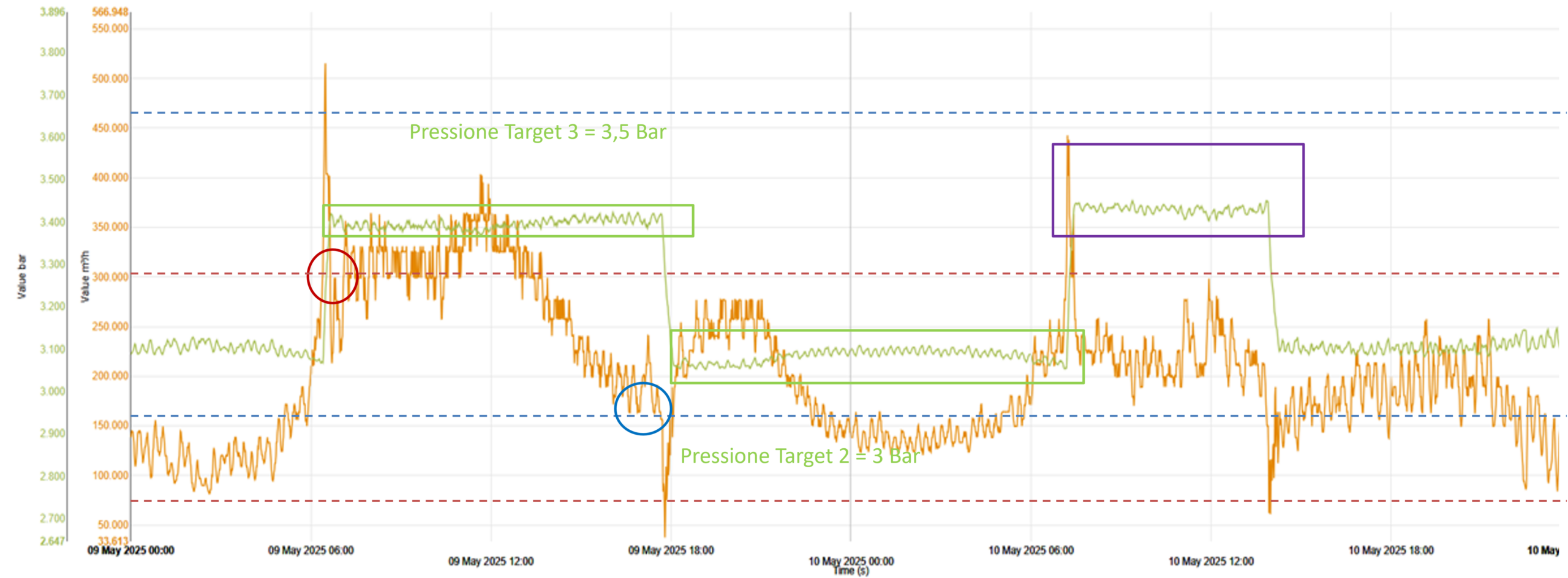
The operating principle of GOLEM-ZERO is based on a flow rate band adjustment. The system divides the network’s operating range into different operating bands, each of which is associated with an optimised target pressure based on demand.
The bands are designed to partially overlap, so as to avoid continuous pressure fluctuations as the flow rate varies. The target pressure is changed only when the flow rate leaves the operating reference band, ensuring operational stability and continuity of service.
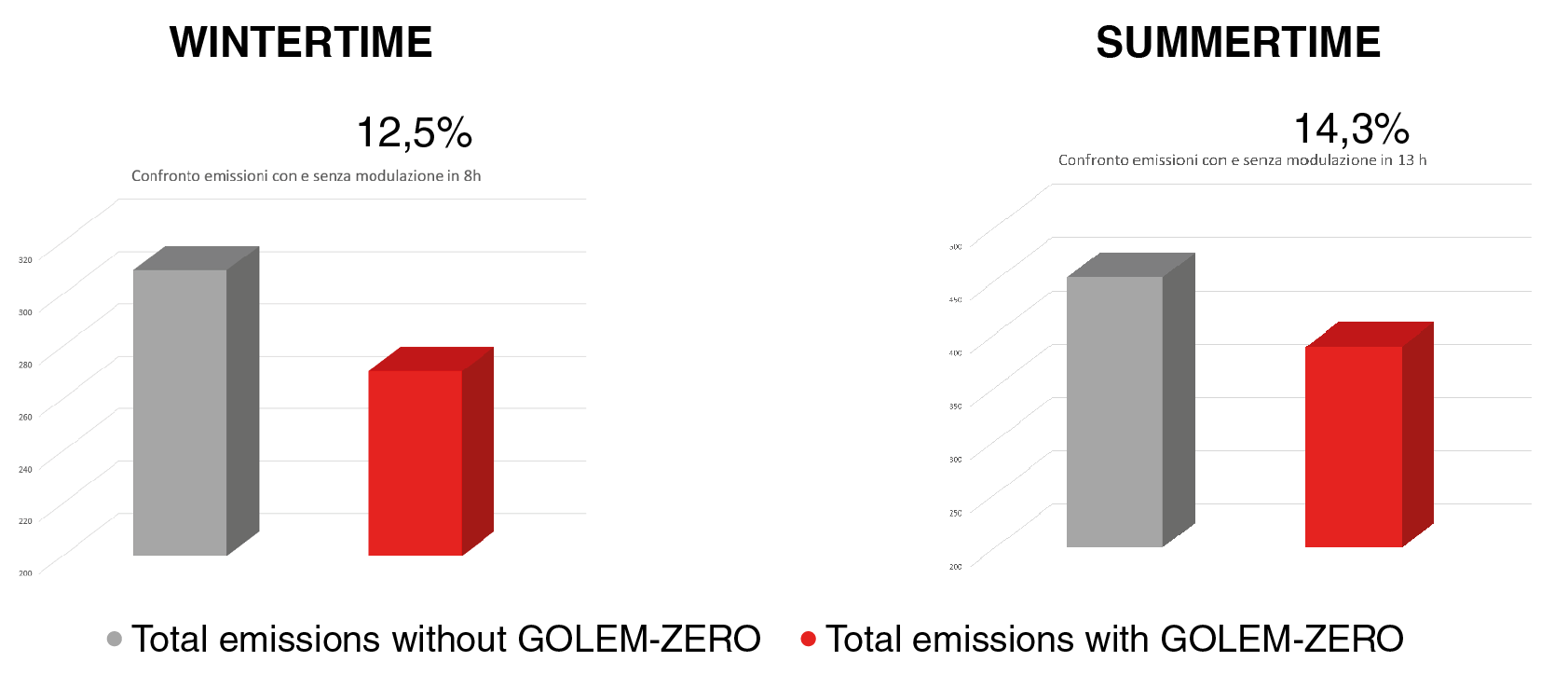
This logic allows GOLEM-ZERO to automatically adapt to different operating conditions — daily, weekly and seasonal — avoiding unnecessary overpressure phenomena. The benefits are also reflected in environmental terms: studies based on models developed by GERG (European Gas Research Group) show reductions in emissions of up to 12.5% in winter and up to 14.5% in summer.
A concrete answer to a real problem
The synergy between MethanEye and GOLEM-ZERO represents a concrete response to the challenges posed by EU Regulation 2024/1787. Not only does it enable methane emissions to be monitored, quantified and reduced, but it also provides operators with a tool to deal with an evolving regulatory environment with greater awareness, reducing operational risk and supporting future compliance.
Tommaso Russo is a Junior Product Manager at AUTOMA S.R.L.. With a degree in Electronic Engineering, he explores new market opportunities and proposes solutions in collaboration with the R&D team. He is also actively involved in promoting AUTOMA’s technologies by delivering technical presentations to potential clients and participating in industry events both in Italy and abroad.
By Cristiano Fiameni, Technical Director of the Italian Gas Committee From the speech ‘Methane emissions: the evolution of legislation’ SMART GRID DAYS 2025, 8 – 9 October 2025.
Methane emissions is a topic we cannot avoid addressing, since EU Regulation 2024/1787 on the reduction of methane emissions in the energy sector has been published. We will therefore see the guidelines along which the activity has developed during 2025 and the prospects we can glimpse in the application phase of this Regulation, which is particularly complex.
The operational challenges of the Methane Emissions Regulation
The Regulation was published in July 2024 and came into force on 4 August of the same year. It is important to emphasise this date, because a series of important deadlines originated from that moment.
This measure is particularity invasive. Indeed, it not only sets the objectives but also maps out the path, leaving little room for the technical sector and causing difficulties from an operational point of view, as it has strong limitations on the modalities that inevitably clash with the practical needs of operators.
As already mentioned, the main objective of the introduction of the Regulation is to reduce emissions; to this end, they must be researched, found, quantified, verified and repaired. Thisapplies to the entire gas chain: transport, distribution, storage and regasification.
On the one hand, covering the entire supply chain is positive. But on the other hand, as the latter is very diverse, the tools to be used should be adapted to each portion of the supply chain. In reality, however, the regulation is one-size-fits-all, and provides a single way of operating regardless of whether one has to work on a regasification plant or on an urban network spread over a city of millions of inhabitants. The requirements and methods of intervention are therefore the same, and this is the crux of the matter from which the critical issues in the application of Regulation 2024/1787 arise.
The fulfilments of the Regulation
Since the entry into force of the Methane Emissions measure, there are several obligations: some are the responsibility of the Member States, while others are the responsibility of the operators or the Commission.
With regard to Member States, several European countries have not yet completed the process of appointing the competent authority. Italy, on the other hand, has already submitted a draft law and made available official e-mails from the MASE (Ministry of the Environment and Energy Security) to which operators can refer for communications.
As mentioned, the operators involved also have certain obligations: in August 2025, for example, they had to submit the first leakage research report (LDAR) on the previous year, and they also had to quantify emissions, using generic emission factors. This meant that even more precise assessments could be made, but the minimum required was the use of literature values of emission factors applied to one’s assets.
The Ministry reported that most operators were able to fulfil this obligation. There will be problems in the coming months, however, because from February 2026 operators will have to submit another report using emission factors specific to their asset. This requires operators to perform an important activity of evaluating their assets, and how to relate this data to factors that have a realistic place in their system. This is not easy so there will be difficulties.
In 2027, however, operators will have to submit a report quantifying emissions from one’s assets and verifying the measures taken on the ground against the results in the atmosphere, i.e., reconciliation. This is a rather ambitious challenge for the sector, given that theRegulation presented the requirements without all the necessary tools being available yet.
The supporting technical standards
Another issue to be taken into account is the instruments, i.e. the technical standards supporting the measure. Indeed, the Regulation not only stipulates that there must be technical standards to support this activity, but also provides that these standards can be recognised by the European Commission as implementing instruments. The body that draws up the standards is the CEN (European Committee for Standardisation), in which several European countries, including Italy, participate.
However, there are critical aspects to this path. The first aspect is that a specific request from the Commission (standardisation request) is needed to draw up standards. This request was submitted in 2024 and it took some time to reach a conclusion. The latest news tells us that the technical phase of discussions between the Commission and CEN has been concluded, and that the contract will be signed shortly. Since the contract provides three years to draft the standards, we could have them by the end of 2028. Therefore, we are faced with an asymmetry: the stricter requirements apply from 2027 onwards, while the standards will perhaps come into force at the beginning of 2028. This represents the first problem.
The second problem is that theRegulation has taken on the honours and burdens of precisely determining technical requirements as well, and this has become an obstacle. Indeed, the Regulation requires the Commission to publish a delegated act specifying the MDLs (Minimum Detection Limits) for technologies and providing guidance on the limits for pre-localisation. The point is that these values have not yet been defined.
An initial stakeholder consultation document came out in 2025, which was supposed to be the basis for producing a subsequent one. The deadline was 5 August 2025, but it was not met. Therefore, we are faced with a doublecritical issue: the first is related to technical standards that are not available due to delays in the Commission’s issuing of the required documents; the second concerns the practical aspect related to operators. The latter, indeed, have obligations that they cannot postpone, and in order to fulfil these obligations they must carry out activities in the field that require investments in technology and equipment.
It must therefore be considered that there are also investments made ‘in the dark’, hoping that industrial best practices will be considered in this delegated act and that consequently these investments will be recognised as valid. Unfortunately, it is a time of great uncertainty.
The work carried out so far and the next steps expected
What have we done in the meantime? The CIG, through the experts made available by its members, participated in the activities and contributed by bringing the Italian position to the European tables.
At European level, it is worth noting the contribution of Marcogaz, the international non-profit association representing the European gas industry, which has produced guidelines for the application of the Regulation. These guidelines provide guidance on the main aspects and introduce two useful elements for operators. Firstly, they provide illustrative diagrams of the process to be followed in accordance with the Regulation. In addition, they include a chapter on the cost-benefit analysis of the activity carried out: the repair of the leak must not cause more environmental damage than the leak itself.
This initial document provides some general guidelines that allow us to assume that this concept will be included in the standardisation request that the Commission will submit to CEN. If this is the case, CEN will be able to develop a chapter dedicated to guidance for operators on cases where the effort is not worthwhile. Especially for those working in the distribution sector, having such indications is very important because the numbers involved are really significant.
Marcogaz in 2024 published guidelines on the Venting & Flaring part and commented in detail on the first consultation paper on the limits proposed by the Commission, which were considered unrealistic for some applications. Indeed, there are both established and modern technologies, but it must be ensured that there is no one way to operate: a neutral approach must be taken in order to achieve the desired result.
In view of the Commission’s request, theCEN decided not to publish the draft on MRV (Monitoring, Reporting, Verification), which started in 2022, but to use it as a technical basis for developing the ongoing standards. The European Technical Committee CEN/TC 234 is developing, in parallel, three standards to support the implementation of the Regulation:
The first is on the quantification of leaks and associated reporting – MRV (Art. 12).
The second is on LDAR (Leak Detection and Repair) (Art. 14).
The third is on Venting & Flaring (Art. 15, Art. 16).
Thus, CEN has already prepared drafts which, in order to be developed and sent to public enquiry, require the two documents we mentioned in the previous paragraphs: thestandardisation request and thedelegated act.
Lastly, the CIG worked on the drafting of a national guideline that, in compliance with legal requirements, would lead to the practical application of the Regulation for the distribution sector, trying to ‘hold together’ the obligations of the provision with the prescriptions of ARERA (Italian Regulatory Authority for Energy, Networks and Environment).
The activity was completed in November 2025 and was preliminarily presented to the MASE.
The Italian Gas Committee, established in 1953, aims to improve safety and efficiency in the use of combustible gases. In 1960, it joined the UNI, the Italian national standardisation body, thus becoming the official Italian body for standardisation in the fuel gas sector.
As an association comprising institutional and non-institutional members, the IGC covers with its members the entire supply chain, from gas import to transport, distribution, storage, utilisation, equipment, devices and installations.
Within the Italian Gas Committee, a federated body of UNI specializing in the field of combustible gases, Eng. Cristiano Fiameni is responsible for technical standardization activities and the development of provided services, including training, seminars, and events.


 Technical Coordinator at INRETE